104
LNG
INDUSTRY
MARCH
2016
but also because the vast majority of machinery data is
uninteresting. One shaft orbit is very similar to the next,
except when problems occur. Therefore, not all vibration
data needs to be saved, but only vibration data that has
changed from the last stored waveform.
This basic idea has existed since the inception of
process historians. It is embodied in the concept of a
deadband, whereby a trend line that is not changing does
not need dozens or hundreds of points stored. It only
needs two points stored, and a straight line drawn
between them. The deadband simply defines how much
change must occur between one point and the next to
recognise it as a new data point, rather than just a linear
extrapolation of the previous data point.
Initially, the primary imperative for deadbands around
process historian points was the limited storage space of
most computers. In the 1980s, when historians were
beginning to debut, a large hard drive was 20 – 40 MB.
Clearly, the ability to store data efficiently was
paramount, and the sophistication of deadbands and
other compression algorithms were likewise paramount.
In a day when a 1 TB drive can be purchased for less than
US$100, it is tempting to think that compression is no
longer that important. There is some merit to this, but
anyone who has ever had to move that 1 TB across a
network will understand that although there is room to
store all of the data, it can take a long time to move it.
Deadbands have historically been used with scalar
data that can be characterised by amplitude and time
tags. However, the concept of only saving data when
something changes can apply to any type of data. It is
now routinely being used by the SETPOINT system to
decide which vibration waveforms to keep and which
ones to ignore.
Consider a shaft turning at 6000 RPM
(100 revolutions/sec.) on a typical compressor train in an
LNG plant. Additionally, assume that the vibration is
sampled 128 times per revolution for 16 shaft revolutions
(waveform consists of 2048 samples with
78 microseconds between each sample). When the
system first turns on (and assuming the machine is
already running at steady-state speed), it stores the
waveform corresponding to those first 16 shaft
revolutions into the historian as a time series, just as with
any other time series data, but with microseconds
between the values rather than seconds, minutes or
hours. It then examines (but does not necessarily store)
the next 16 shaft revolutions (revolutions 17 – 32). It
examines multiple attributes of the waveform, such as
overall amplitude, gap voltage, frequency content, period
(machine speed), etc., and compares these to similar
attributes of the initial 16 revolutions already stored. If
things have adequately changed, it also stores the new
waveform. If things have not adequately changed, it only
keeps the first waveform and discards the other. The
system continues on in this way indefinitely, collecting
and examining every waveform, but only saving those
that represent sufficient change from the baseline. This, in
essence, is how the deadbanding of waveforms, rather
than just scalar data, is accomplished.
By utilising the concept of a deadband for not only
conventional trend data, but also for high speed
waveform data, the system is able to continuously collect
and analyse every waveform from every rotation of the
machine’s shaft. However, it only stores this data when a
waveform has sufficiently changed relative to its
constantly updating baseline. The system can, therefore,
go for long intervals without saving extraneous
waveforms if conditions are not changing, yet store
waveforms quickly when conditions are rapidly changing,
such as during machine start-ups, process upsets, or
incipient mechanical failures. Therefore, two years of data
from a typical 300-channel system only requires a modest
1 TB of storage space, employing a combination of
compression algorithms native to the process historian
and new algorithms for high speed waveform data.
Boost mode
Some machines can exhibit extremely fast starts
and stops, such as motor driven pumps and smaller
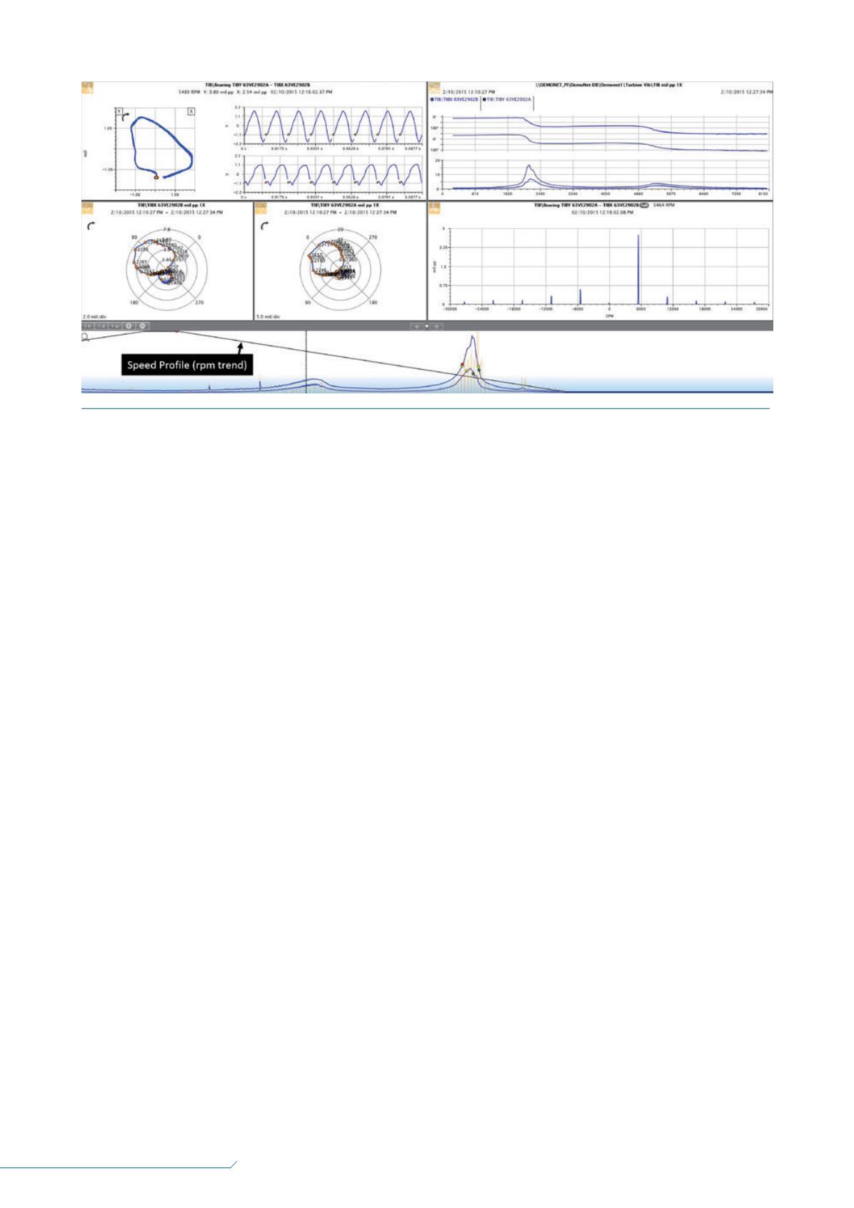
Figure 5.
Waveform data collected during a machine trip.


